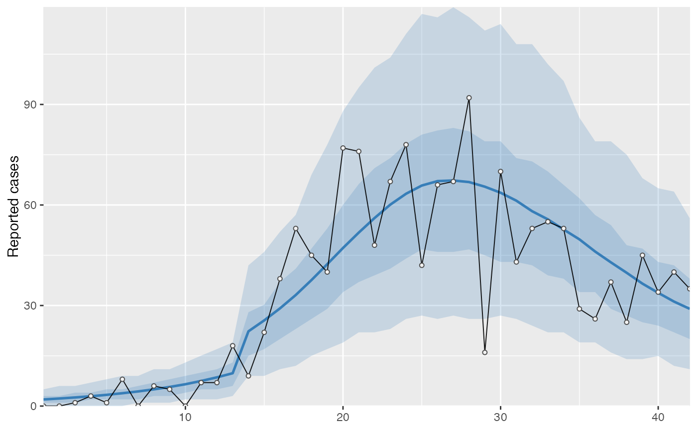
Make a projection with a SEIR fit — project

Predict from a fit_seir() object, possibly with a future prediction. By default, the projection uses the estimated f values (fraction of normal contacts encountered for those physical distancing). The function also includes functionality to specify a vector of fixed f values starting on a given future date.

project_seir(
  obj,
  forecast_days = 0,
  f_fixed_start = NULL,
  f_fixed = NULL,
  f_multi = NULL,
  f_multi_seg = NULL,
  iter = seq_along(obj$post$R0),
  return_states = FALSE,
  imported_cases = 0,
  imported_window = 1,
  parallel = TRUE,
  X = obj$stan_data$X,
  ...
)

Arguments

obj	Output from `fit_seir()`.
forecast_days	Number of projection days.
f_fixed_start	Optional day to start changing f. Must be set if `f_fixed` or `f_multi` is set. This is the day number to start, not the number of days into the projection. E.g., if 100 days were fitted to and `f_fixed` should start 5 days into the future, then `f_fixed_start = 105`.
f_fixed	An optional vector of fixed f values for the projection. Should be length `forecast_days - (f_fixed_start - nrow(daily_cases) - 1)`. I.e. one value per day after `f_fixed_start` day.
f_multi	Multiplicative vector of f values. Same structure as `f_fixed`.
f_multi_seg	Which `f` to use for `f_multi`.
iter	MCMC iterations to include. Defaults to all.
return_states	Logical for whether to return the ODE states.
imported_cases	Number of cases to import starting on first projection day.
imported_window	Number of days over which to distribute imported cases.
parallel	Use parallel processing via future and furrr?
X	An optional model matrix that acts additively on log expected cases.
...	Other arguments to pass to `rstan::sampling()`.

Value

A data frame:

day: Day
data_type: Data-type column from the case data
mu: Expected number of cases
y_rep: Posterior predictive replicate observation
phi: Posterior draw of phi, the NB2 dispersion parameter, if included
.iteration: The MCMC iteration

Details

Set a future::plan() and this function will operate in parallel across MCMC iterations using future and furrr.

Examples

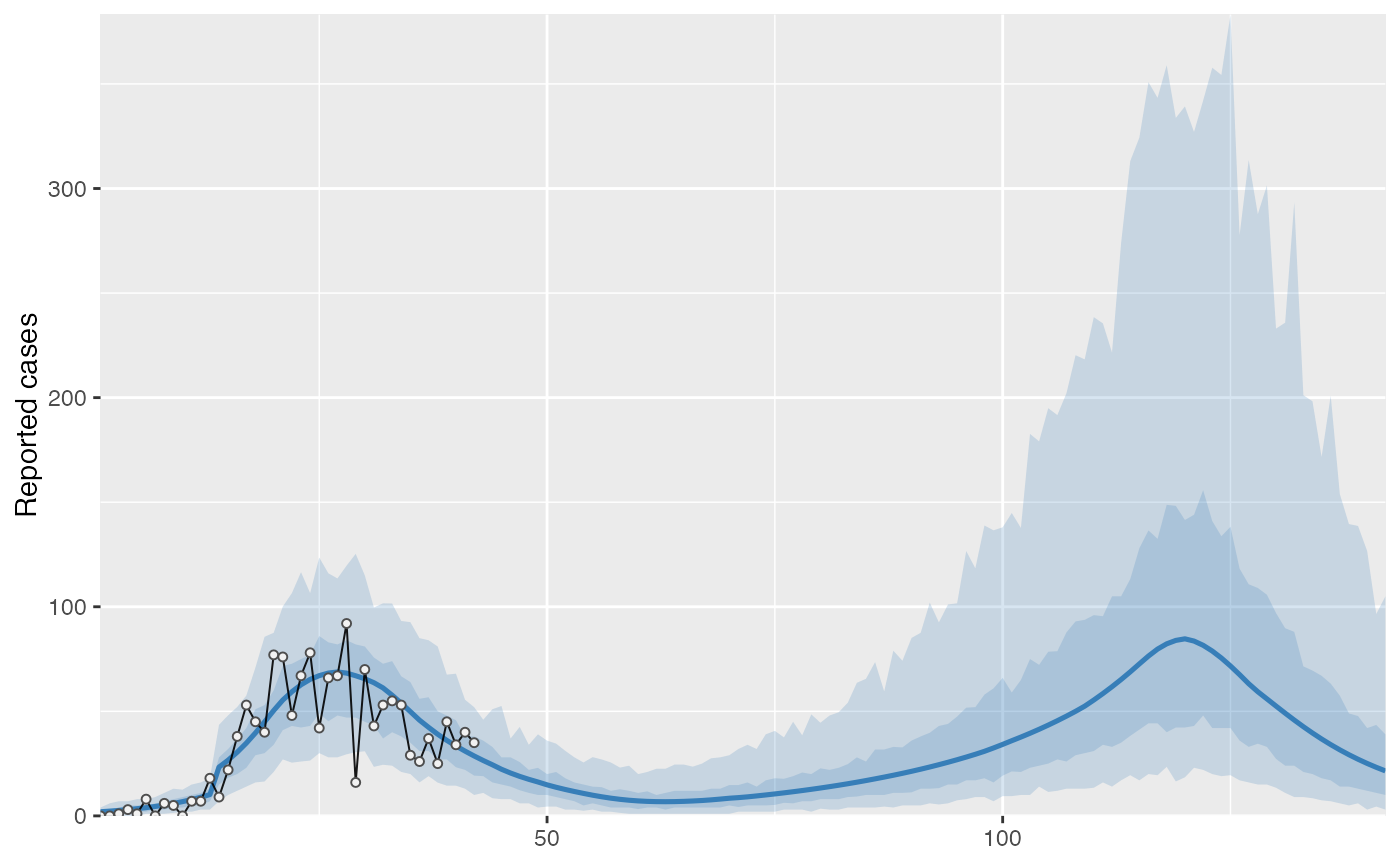
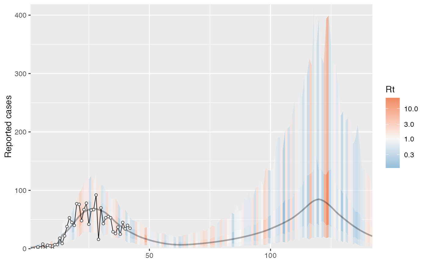
cases <- c(
  0, 0, 1, 3, 1, 8, 0, 6, 5, 0, 7, 7, 18, 9, 22, 38, 53, 45, 40,
  77, 76, 48, 67, 78, 42, 66, 67, 92, 16, 70, 43, 53, 55, 53, 29,
  26, 37, 25, 45, 34, 40, 35
)
# Example fixed sample fractions:
s1 <- c(rep(0.1, 13), rep(0.2, length(cases) - 13))

# To use parallel processing with multiple chains:
# options(mc.cores = parallel::detectCores() / 2)

# Using the MAP estimate for speed in this example:
m <- fit_seir(
  cases,
  iter = 100,
  i0_prior = c(log(8), 0.2),
  samp_frac_fixed = s1,
  fit_type = "optimizing"
)
#> Finding the MAP estimate.
print(m)
#> MAP estimate:
#>            i0            R0 start_decline   end_decline        f_s[1] 
#>          7.33          3.13         14.82         21.58          0.22 
#>        phi[1]             e 
#>          6.48          0.82 
#> Mean in constrained space of MVN samples:
#>            i0            R0 start_decline   end_decline        f_s[1] 
#>          7.40          3.14         14.82         21.54          0.23 
#>        phi[1]             e 
#>          7.23          0.83 
#> SD in constrained space of MVN samples:
#>            i0            R0 start_decline   end_decline        f_s[1] 
#>          1.39          0.10          0.60          0.92          0.09 
#>        phi[1]             e 
#>          2.64          0.05 

p <- project_seir(m)
p
#> # A tibble: 4,200 x 7
#>      day data_type    mu y_rep   phi .iteration forecast
#>    <int>     <int> <dbl> <dbl> <dbl>      <int> <lgl>   
#>  1     1         1  1.73     2  10.1          1 FALSE   
#>  2     2         1  1.99     0  10.1          1 FALSE   
#>  3     3         1  2.28     3  10.1          1 FALSE   
#>  4     4         1  2.61     1  10.1          1 FALSE   
#>  5     5         1  3.00     6  10.1          1 FALSE   
#>  6     6         1  3.44     4  10.1          1 FALSE   
#>  7     7         1  3.94     4  10.1          1 FALSE   
#>  8     8         1  4.52     4  10.1          1 FALSE   
#>  9     9         1  5.18     4  10.1          1 FALSE   
#> 10    10         1  5.94     2  10.1          1 FALSE   
#> # … with 4,190 more rows

obs_dat <- data.frame(day = seq_along(cases), value = cases)

library(magrittr) # for %>%
#> 
#> Attaching package: ‘magrittr’
#> The following object is masked from ‘package:purrr’:
#> 
#>     set_names
tidy_seir(p) %>% plot_projection(obs_dat = obs_dat)

tidy_seir(p) %>%
  plot_residuals(obs_dat = obs_dat, obj = m)

# for parallel processing (optional)
# future::plan(future::multisession)
p <- project_seir(m,
  forecast_days = 100,
  f_fixed_start = 53,
  f_fixed = c(rep(0.7, 60), rep(0.2, 30)),
  iter = 1:25
)
p
#> # A tibble: 3,550 x 8
#>      day data_type    mu y_rep   phi .iteration forecast f_fixed
#>    <int>     <int> <dbl> <dbl> <dbl>      <int> <lgl>    <lgl>  
#>  1     1         1  1.73     2  10.1          1 FALSE    FALSE  
#>  2     2         1  1.99     1  10.1          1 FALSE    FALSE  
#>  3     3         1  2.28     3  10.1          1 FALSE    FALSE  
#>  4     4         1  2.61     2  10.1          1 FALSE    FALSE  
#>  5     5         1  3.00     3  10.1          1 FALSE    FALSE  
#>  6     6         1  3.44     1  10.1          1 FALSE    FALSE  
#>  7     7         1  3.94     5  10.1          1 FALSE    FALSE  
#>  8     8         1  4.52     2  10.1          1 FALSE    FALSE  
#>  9     9         1  5.18     3  10.1          1 FALSE    FALSE  
#> 10    10         1  5.94     6  10.1          1 FALSE    FALSE  
#> # … with 3,540 more rows
tidy_seir(p) %>% plot_projection(obs_dat = obs_dat)

# fake example to show optional Rt colouring:
proj <- tidy_seir(p)
plot_projection(proj, obs_dat = obs_dat, Rt = rlnorm(nrow(proj)), col = "#00000050")


# Get threshold for increase:
# future::plan(future::multisession) # for parallel processing (optional)
# (only using 40 iterations for a fast example)
thresh <- get_threshold(m, iter = 1:40, show_plot = TRUE)
#> Projecting 0.3 
#> Projecting 0.47 
#> Projecting 0.63 
#> Projecting 0.8 
mean(thresh)
#> [1] 0.5571626

# Get doubling time (prevalence is declining in this example)
get_doubling_time(m, iter = 1:40, show_plot = TRUE)
#>  [1] -12.206996  -9.120015 -12.842758  -9.945963  -7.811543  -6.515639
#>  [7]  -7.816685  -5.760329 -13.761678 -10.993012  -7.416578  -9.105512
#> [13] -17.026427 -12.731450  -8.465330  -6.481328  -6.337543  -7.559904
#> [19]  -8.182519  -7.880885  -6.774119  -8.785315  -9.527219  -8.329275
#> [25] -10.806046  -8.668513  -7.900398 -35.571056  -6.880035  -9.164080
#> [31]  -6.748669  -9.830272  -7.800595  -8.795443  -8.114695 -14.976421
#> [37] -13.397818  -6.696756 -15.460064  -8.028927

states_with_Rt <- get_rt(m)
states_with_Rt
#> # A tibble: 28,900 x 15
#>    .iteration  time       S    E1    E2     I       Q       R     Sd   E1d   E2d
#>         <int> <dbl>   <dbl> <dbl> <dbl> <dbl>   <dbl>   <dbl>  <dbl> <dbl> <dbl>
#>  1          1 -30    1.58e6 0.723 0.181 0.904 4.52e-8 1.81e-7 3.52e6  1.61 0.403
#>  2          1 -29.8  1.58e6 0.828 0.175 0.893 1.10e-2 4.52e-2 3.52e6  1.85 0.391
#>  3          1 -29.5  1.58e6 0.926 0.175 0.881 2.12e-2 9.03e-2 3.52e6  2.06 0.391
#>  4          1 -29.2  1.58e6 1.02  0.180 0.870 3.09e-2 1.35e-1 3.52e6  2.27 0.401
#>  5          1 -29    1.58e6 1.10  0.187 0.862 3.99e-2 1.81e-1 3.52e6  2.46 0.417
#>  6          1 -28.8  1.58e6 1.19  0.196 0.856 4.85e-2 2.26e-1 3.52e6  2.65 0.438
#>  7          1 -28.5  1.58e6 1.27  0.207 0.853 5.65e-2 2.71e-1 3.52e6  2.82 0.462
#>  8          1 -28.2  1.58e6 1.34  0.219 0.853 6.42e-2 3.17e-1 3.52e6  3.00 0.489
#>  9          1 -28    1.58e6 1.42  0.232 0.856 7.14e-2 3.63e-1 3.52e6  3.16 0.517
#> 10          1 -27.8  1.58e6 1.49  0.245 0.862 7.84e-2 4.10e-1 3.52e6  3.33 0.546
#> # … with 28,890 more rows, and 4 more variables: Id <dbl>, Qd <dbl>, Rd <dbl>,
#> #   Rt <dbl>

library(ggplot2)
ggplot(states_with_Rt, aes(time, Rt, group = .iteration)) +
  geom_line(alpha = 0.5)
#> Warning: Removed 12000 row(s) containing missing values (geom_path).